Adaptive Cubic Convolution Of High Resolution Remotely Sensed Image Data

Adaptive Cubic Convolution Of High Resolution Remotely Sensed Image Data

Raveentheran Suntheralingam
Sime Darby Systems, Wisma Sime Darby
Jalan Raja Laut, 50490 Kuala Lumpur, Malaysia
E-mail: rsl@sds.po.my

Abstract
Cubic convolution of high resolution Airborne Thematic Mapper (ATM) images usually result in overshoot artefacts that are created on either side of boundaries or edges between spectrally different entities. The severity of these artefacts has previously been minimised by applying hybrid techniques that involve resampling by nearest neighbour assignment across edges, and cubic convolution in other regions of the image.

It is suggested that a form of cubic convolution that modifies its a and b parameters across an edge can be used to resample A TM images. In this scheme, an edge within a cross-section of an A TM image is firstly identified. Values of a and b that generate resampled grey level values obtained by nearest neighbour assignment are evaluated for each pixel across the edge. Experimental results are used to show that linear relationships exist between a and b for each pixel across the selected edge, suggesting that this adaptive cubic convolution scheme can be used to resample edges in A TM images.

I. Introduction
In most remote sensing applications, images are frequently resampled and subsequently interpolated by the nearest neighbour assignment, bilinear interpolation or cubic convolution resampling techniques. Each of these resampling schemes generate artefacts and introduce a characteristic comlption into the resampled image. Nearest neighbour assignment, for example, tends to degrade the structure of the image, but is particularly useful for resampling edges. Cubic convolution introduces overshoots at image edges, but depending on its parameters, can geoorate acceptable resampled images.

It is desirable to resample edges in high resolution images by cubic convolution without creating any overshoots. One approach is to use different interpolators to resample across an edge Devereux et al. 1989]. This hybrid form of resampling can, for example, use nearest neighbour assignment to resample across edges thereby eliminating overshoot artefacts, and cubic convolution to resample other regions in the image. However if the cubic convolution function can be made to preserve grey level values across edges in the same way as nearest neighbour assignment, it would not be necessary to use hybrid schemes to resample A TM images. In this paper, it will be shown that cubic convolution parameters that do not generate overshoot can be evaluated thereby suggesting that an adaptive form of cubic convolution that uses different parameters can be used to resample across edges. This paper is organised as follows. The relationship between cubic convolution parameters, and the resulting overshoots is presented in section 2. Estimation of these parameters that generate minimal overshoot is outlined in section 3. Conclusions are drawn in section 4.

2 Analysis of Overshoots Generated by Cubic convolution
Cubic convolution calculates resampled pixel grey level values from sets of sixteen neighbouring pixels in the original image (four along the x-direction) by using a reconstruction kernel that was expressed by Reichenbach and Park [1989] as,

where

Here, the value of the first derivative of the kernel, and the value of the kernel at I are represented by the a. and paramete respectively .The cubic convolution function is continuous and symmetrical, and satisfies the concavity conditions of being concave upward at x = 0, and concave downward at I x = I when -3 < a. < 0 (with 13 = 0) (Bernstein 1976]. A severe shortcoming of cubic convolution however, is its tendency to create overshoots on either side of resampled edges. Previous work on cubic convolution by Keys (1981], Park and Schowengerdt (1983], and Mitchell and Netravali (1988] showed that the magnitude of these artefacts and quality of resampled low resolution images clearly depended on the values of a. and 13.

It is desirable to establish the relationship between a. and 13, and the magnitude of overshoot that it generates in order to develop a cubic convolution scheme that minimises the severity of these artefacts. This relationship is best illustrated by unifomlly resampling one-dimensional arrays of integers representing grey level values of selected cross-sections of test or real image data. Subtle changes in resampled grey level values, which would otherwise be unnoticeable in resampled images can be easily observed. Results presented in this section are based on resampling a synthetic edge comprising 24 integers with values { 50, 50, 50, 50, 50, 200, 200, 200, 200,200, 185, 170, 155, 140, 125, 110, 95, 80,65, 50, 50, 50, 50, 50 }. These integer values were deliberately selected to represent the steep edge and gradual variations in grey level values found in remotely sensed images. The test data set was resampled at 25 equally spaced intervals for a range of a. and 13 values. Percentage overshoot generated at specific pixel positions around the steep edge in the resampled test data set were calculated as~where q and p denotes pixel grey level values before and after resampling respectively .

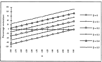
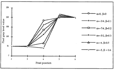
The percentage overshoot generated at pixel position 3 (with q = 50) for a range of values of a. (with 13 kept constant) is illustrated in figure I. It can be seen that percentage overshoot at pixel position 3 increases linearly with a., and that there exists several values of a. and 13 which do not generate any overshoot. Sets of 0. and 13 values that generate zero percentage overshoot at pixel position 3 were used to resample the original test data set at 25 equally spaced intervals. Figure 2 shows the grey level values generated between pixel positions 2 and 6 for these combinations of a. and 13 values. It can be seen that overshoots are not found at pixel position 3 for the different values of a. and 13 that were used. However a large range of grey level values are observed at pixel position 4. Smaller variations of grey level values are noted at pixel position 5.

Figure 1: Plot of percentage overshoot at pixel position 3. Values of @ and @ that generate zero percentage overshoot can be found.

Figure: 2 Plot of grey level values for @ and @ that generate zero percentage overshoot at pixel position 3. A large range of grey level values are observed at pixel position 4. Smaller variations of grey level values occur at pixel position 5.
It has been shown that specific values of a. and 13 can be found to minimise overshoot or undershoot at certain pixel positions. This is achieved however at the expense of excessive smoothing or poor reconstruction generated at other pixel positions. These results also suggest that cubic convolution at specific pixels on either side of edges can be achieved without generating any overshoot at the particular pixel if appropriate values of a. and 13 can be found. Consequently, it would seem that if a. and 13 can be appropriately modified across the edge, cubic convolution can be applied to resample edges without generating any overshoot or undershoot.

3. Estimation of Cubic Convolution Parameters
Hybrid resampling techniques by Devereux et al. (1992] involved the use of different resampling schemes at different regions within an image. The image data set that was used to generate the results presented in this section was acquired from the cross-section of an ATM image. This data set is illustrated in figure 3, and comprises 35 integers with grey level values typical of 4 meter resolution images captured at 1.55J.lm to 1.75J.lm. A steep edge between the darker forest region and lighter grassland is located at pixel position 14. Table I shows the differences between the grey level values obtained by applying cubic convolution to resample the entire A TM image data set, against those obtained from nearest neighbour assignment within two pixels of the edge and cubic convolution for all other pixels. Cubic convolution in both cases was achieved with a. = -0.5 and 13 = 0.056. It can be seen that a large difference in grey level value exists at pixel position 12.

Table 1 : Grey level values obtained by hybrid resarnpling and cubic convolution of the entire A TM image data set. Differences in grey level values are observed between pixel positions 11 and 16.

Pixel position	8	9	10	11	12	13	14	15	16	17	18
Cubic convolution of entire ATM data set	47	81	86	17	62	211	215	203	189	177	197
Hybrid resarnpling	47	81	86	20	195	215	205	191	189	177	197

Figure 3: Cross-section of ATM image. Pixel position 1 to 11 represent forest. Positions 14 to 35 represent grassland. Significant variations in grey level values are typical of high resoulution ATM images.
If p_n-l, p_n p_n+l and p_n+l represent pixel values in the original data set, the resampled grey level value between pixel values p_n and p_n+l is estimated by cubic convolution as,

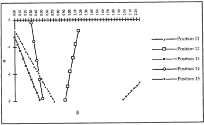
where |xi| is the distance from the resampled pixel position to the nearest neighbouring pixel in the original data set. The resampled grey level values 20, 195, 215, 205 and 191 generated by the hybrid resampling scheme for pixel position 11, 12, 13, 14, and 15 respectively can be obtained by cubic convolution for appropriate values for a and b If P r is given the grey level value obtained by the hybrid resampling scheme, appropriate values of a and can be evaluated by parametrically solving equation 4. Figure 4 shows the set of a and b values that generate grey level values 20, 195, 215, 205 and 191 at pixel positions 11 to 15. It can be seen that linear relationships exist between a and b Equations of lines relating a and b are evaluated by coordinate geometry and shown in table 2. These linear relationships indicate that different combinations of a and b values can be used to generate the same grey level value. In order to select acceptable values for a and b it is essential to ensure that the resulting cubic convolution functions for these values of a and b meet the necessary concavity conditions.

Table 2 : Relationships between a and b that generate grey levels obtained by nearest neighbour assignment.

Pixel	Range for a	Range for b	Relationship	a	b
11	1.16<a<-0.18	-0.06<b<0.20	a=-3.7b-0.4	-0.4	0
12	65.22<a<5.04	7.58<b<1.68	a=10.2b-12.1	-0.4	1.15
13	-1.47<a<-0.22	-0.07<b<0.17	a=-5.2b-0.6	-0.9	0.05
14	-0.22<a<0.72	0.24<b<0.31	a=-14b+4.1	-0.1	0.3
15	-20.41<b<7 .89	-6.80<b<0.54	a=2b-6.8	-8.0	-0.6

Figure 4: Set of a and b values that generate the grey level values obtained by nearest neighbour assignment. Linear relationships are observed to exist between @ and @.
The concavity conditions, -3 < a < 0, described by Bernstein [1976] are inadequate to establish suitable ranges of values for a and b for the adaptive cubic convolution technique since these conditions only apply to the case when x = 0. It is therefore desirable to use more appropriate concavity conditions that can be applied to select acceptable values of a and b as shown in equation 5 Suntheralingam 1994].

9b -3 < a < 3b (5)
These more general concavity conditions are used to evaluate appropriate ranges for a and b that generate the grey level values obtained by nearest neighbour assignment. The equations of the lines shown in figure 4 are expressed as functions of a and b, and substituted into equation 5. The resulting range of values for a and b that satisfy the necessary concavity conditions are shown in table 2. Cubic convolution of the A TM image data set using the selected a and b values also shown in table 2 were found to generate grey level values 20, 195, 215,205 and 191 for pixel positions II to 15. These results demonstrate that cubic convolution is capable of generating the same grey level values that are obtained by nearest neighbour assignment.

4. Summary and Conclusions
The suitability of resampling edges in ATM image data by an adaptive form of cubic convolution that appropriately modifies its parameters across the edge has been demonstrated by experimental results presented in this paper. It has been shown that values for a and b can be evaluated to resample edges in ATM images without generating overshoots. The one-dimensional approach adopted in this paper ignored the effects of other neighbouring pixels in the image apart from those found along the recorded cross-section. In reality however, all neighbouring pixels around a resampled point within an image clearly influence the resampled grey level estimate. Further work therefore needs to be carried out to extend the adaptive cubic convolution technique to two-dimensions.

The major problem associated with adaptive cubic convolution is the difficulty in estimating suitable values of a and b for different regions in an image. Since the values of a and b are scene dependent, a simple and effective model that relates these parameters to some characteristic about the image needs to be developed. Schowengerdt et al. [1984] suggested the possibility of using local image frequency content to evaluate suitable values for the cubic convolution parameters. Visual examination shows that A TM images tend to be fairly textured. It would therefore be interesting to establish whether the local frequency content within the A TM image is related to image texture. If image texture is found to be an appropriate measure of frequency content, any texture analysis that is required to evaluate a and b is likely to impose a significant computational overhead. Adaptive cubic convolution in such a case would therefore be useful only if coupled with a very fast algorithm for estimating a and b, otherwise any increase in the image quality of the resampled image would be negated by a significant increase in computational effort.

5. References

Bemstein R ( 1976) Digital image processing of earth observation sensor data. IBM Journa/ of Research and Deve/opment 20(1):40-57.
Devereux B J, Fuller R M, Roy D P ( 1989) The geometric correction of Airborne Trematic Mapper imagery . Proceedings of the NERC workshop on Airborne Remote Sensing, Windermere, pp 19-33.
Devereux B J, Roy D P, White S J, Fuller R M, Hopper F (1992) Cartographic Registration of Airborne Remote/y Sensed Data. NERC Research Contract Report F60/G6/28.
Keys R G (1981) Cubic convolution interpolation for digital image processing. free Transactions on Acoustics, Speech and Signa/ Processing 29(6): 1153-1160.
Mitchell D P, Netravali AN (1988) Reconstruction filters in computer graphics. Computer Graphics 22(4):221-228.
Park S K, Schowengerdt R A (1983) Image reconstruction by parametric cubic convolution. Computer Vision, Graphics and Image Processing 23(3):258-272.
Reichenbach S E, Park S K (1989) Two-parameter cubic convolution for image reconstruction. Proceedings of the SPIE, Visua/ Communications and Image Processing IV 1199:833-840
Schowengerdt R A, Park S K, Gray R (1984) Topics in the two-dimensional sampling and reconstruction of images. Internationa/ Journa/ of Remote Sensing 5(2):333-347.
Suntheralingam R (1994) Developments in image resampling techniques. MPhi/ thesis, Cambridge University..