| GISdevelopment.net ---> AARS ---> ACRS 1995 ---> Spatial Information Processing |
GA Optimization Technique On
Spatio-Temporal Interpolation For Dynamic GIS
Shaobo Huang* and Ryosuke
Shibasak**
*Center for Environmental Remote Sensing,
Chiba University, Japan
E-mail : shaobo@rsirc.cr.chiba-u.ac.jp
**Institute of Industrial Science,
University of Tokyo, Japan
E-mail : shiba@shunji.iis.u-tokyo.ac.jp
Abstract *Center for Environmental Remote Sensing,
Chiba University, Japan
E-mail : shaobo@rsirc.cr.chiba-u.ac.jp
**Institute of Industrial Science,
University of Tokyo, Japan
E-mail : shiba@shunji.iis.u-tokyo.ac.jp
Generating cross-sectional data of arbitrary time slice is a basic function to support temporal operations such as time-series analysis and integration of dynamic models in Global GIS environment. To generate time slice data, it is necessary to interpolate/integrate existing global data with different temporal coverage and spatial resolution. Although interpolate/ integrate methods have been developed for continuous variable data, there are only very primitive interpolation methods such as nearest neighbor interpolation considered about class variable data. Here we proposed a spatio-temporal interpolation scheme for pixel-based class variable data under the framework of optimization of likelihood. To optimize the likelihood of spatio-temporal data, a Genetic-Algorithm Hill-Climbing model (GA/HC), which combined genetic-algorithm and Hill-climbing method together to increase the efficiency and quality of optimization, was developed. In GA/HC, a direct coding method and new reproduction and crossover operators are proposed for 3D spatio-temporal data. The evaluation function of GA/HC is defined in the respect to the effect of neighboring spatial-temporal relations on the class change. Through several testing experiments, it showed that GNHC can be a good spatio-temporal interpolation.
1. Background and Objective of the Study
Temporal or dynamic analysis of spatial data are needed in various fields such as environmental systems analysis. One of the most fundamental problems which users are facing is the difficulties in generating spatio-temporal filed of quality data for analysis through an interpolation or integration of observational data. In several fields, to improve reliability of spatio-temporal interpolation/ extrapolation in generating quality data, models and/or equations describing an underlying mechanism and structure is integrated with observational data. By integrating observational data and models describing underlying mechanisms and structures of object-phenomenon with a GIS, we can provide a GIS-based environment which allow dynamic update of spatio-temporal field of data whenever a new observational data and an improvement of models are given. If computational speed for integration is fast enough, we can store only observational data and can estimate data at any locations based on the requests.
Integration methods for data and models have been mainly developed for continuous variables in meteorology and oceanography such as temperature and precipitation. For categorized or class variables such as land use types, there is only very primitive interpolation methods such as nearest neighbor interpolation and so forth. In this paper, the authors propose a integration methods of models and class data from multi-sources under the framework of optimization of likelihood of spatio-temporal events. For optimizing the likelihood, genetic algorithm (GA) is modified by combining GA with classical "Hill climbing" method. Experimental results demonstrate that GA can be successfully applied to the integration.
2. Genetic Algorithm (GA) and Class Variable Interpolation
2.1 Introduction of Genetic Algorithm (GA)
Genetic algorithms are developed by John Holland and his colleagues as an approach to optimization which requires efficient and effective search in natural and artificial systems. They are search algorithms based on the mechanism of natural selection and evolution of natural genetics. They combine survival of the fittest among string structures with a structured but randomized gene exchange to form a search algorithms with some of innovative flair of human search (D.E.Goldberg, 1989).
Genetic algorithms are computationally simple and powerful in their search without restrictive assumptions about search spaces. In a simple genetic algorithm, five basic aspects should be considered: the representation or coding of problem, the initialization of population, the definition of evaluation function, the definition of genetic operators, and the determination of parameters.
2.2 Optimization Scheme for Class Variable Interpolation
Most natural properties may vary continuously. However, the observation that describe these, properties and which form the data bases of GISs are usually fragmentary .Ever where a complete cover of information exists, for instance from the satellite images, we still often need to resample because there are too many data to handle or analyze in any reasonable time. Because the properties are continuous that values in sites are close together in space are more likely to be similar than those further from one another, i.e., they depend on one another in a statistical sense. This important feature of spatial data provides the rationale for interpolation (M.A.Olover, 1990).
Spatial-temporal data can be divided into two types: continuous variables data and class variables data R.Shibasaki et.al.(1993). proposed a Kriging-based integrating/interpolation method for continuous variable data and an interpolation method for class variable data based on the estimation of time of changes according to "class boundary distance". But for the class variable data, the method of the time-of-change estimation seems not to work well, because complex temporal and spatial relations among classes around a pixel greatly affect class variation at this pixel and make it difficult to estimate the time of change at the pixel. In fact, interpolation problem of class variable data is a hardest combinatorial optimization problem in spatial and temporal dimensions.
In this research, we go to integrate observational class data with behavioral/structural models/rules to make robust and reliable spatio-temporal interpolation of class variables. Since searching for the most likely spatio-temporal field of class data is typical combinatorial optimization problem, we introduce the genetic algorithm as a optimization scheme for class variable data to get optimized interpolated time-slice data. To estimate the most likely spatio-temporal field of class data, we maximize the likelihood of estimated spatio-temporal field. The likelihood is computed based on both the fitness to observational data and that to behavioral/structural models/rules. The fitness to observational data is determined from the accuracy and resolution of observational data, while the fitness to behavioral/structural models/rules is computed as the combined likelihood(probability) of transitional events under the assumption that all transitions follow probabilistically the behavioral/structural models/rules.
3. Application of Genetic Algorithm for Integrating Behavioral Models and Observational Data to Class Variable Interpolation
3.1 3D Representation of an Individual (coding)
In the research, two dimensional spatial and one dimensional temporal space was considered to compose a 3D spatio-temporal space as shown in Figure.1, in which horizontal surface is used to represent 2D space and vertical dimension is used to represent temporal dimension. A three dimensional array is defined to represent the individual.
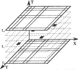
Figure 1 Representation of Individual
3.2 Initialization of Population
An initial population for a genetic algorithm is usually chosen at random; one random trial is made to produce each individual. All members of initial population are chosen automatically by same procedure so that the expected value of each member of initial population is same. In addition we use cubes of 1 * 1 * 1, 2*2*2 and 3*3*3 pixels as the initial unit for the initialization of population to increase the efficiency of algorithm.
3.3 Definition of Individual's Fitness
3.3.1 Spatio-temporal Behavioral Models/Rules of Class Variable Data
It should be noted that any types of behavioral/structural models/rules can be used for the GA-based interpolation if they can determine the probability of every possible behavior/transition of class variables. In class variable data, the possible changes of a class at one pixel is basically defined by the probability of the changes from one class to another. One of the simplest example is a Markov chain, where transitional probability is determined only by the previous class. In addition the probability also can be affected by combination of classes in the neighborhood. In this study, we assume the transitional probability is determined by the combination of classes in the neighborhood. And landuse data with five classes is used as test data.
The spatial and temporal relations affect the transitional probability in three ways as shown in the Figure.2. The first is so-called the spatial continuity, which is based on the assumption that the same class data tends to continue in spatial dimension. Therefore, the effects of the spatial relation happen just within the same time-slice data. Second one is called temporal continuity .This is an extension of spatial continuity to temporal domain- The third aspect is expansion-contraction relations based on the assumption that some class data has high possibility to expand its area at next time-slice, while others tend to contract. The temporal change in the pixel with un-contractible class type will be determined by the pixel' s class itself. And the temporallanduse change in the pixel with contractible type will be determined by class of the pixel and classes of its expandable neighborhood.
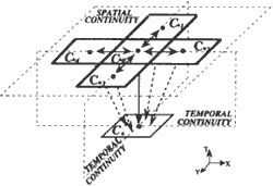
Figure 2 3D Spatial-Temporal Relation of Pixel-based Class Variable Data
3.3.2. Calculation of Individual's Fitness
Individual's fitness has two parts: behavioral fitness and observational fitness. Behavioral fitness is defined as combined probability of change events of class variables when these changes follow probabilistic behavioral models or rules. Observational fitness can be defined as combined probability that the observational class values occur under probabilistic functions of observational errors I uncertainties. By multiplying behavioral fitness and observational fitness, overall fitness can be computed. To integrate behavioral/structural models and observational data, the overall fitness have to be optimized. In this paper, we omit the observational fitness just for simplification of simulation.
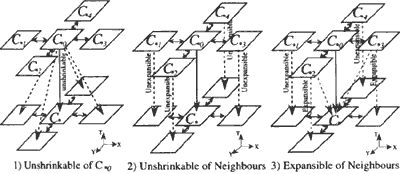
Figure 3 Possible Class Change in 3D Spatio-temporal Space
Figure.3 shows possible class change in spatio-temporal space. Let define PTC(C*0,C.) as the probability of class change from class C*o to class C. by temporal continuity under the effect of expansion- contraction within C*o, 's neighbourhood and psc (C*o ~ C.) as the probability of class change by spatial continuity. If it is assumed that PTC(C*o, C.) and Psc(C.o -C.) are independent, we can compute behavioral fitness of each individual according to following formula:

where Np is the pixel number
NT : is the temporal slice number,
CP, T : is the landuse class of the cell on the Pth pixel at the T time slice;
For the class change probability with spatial continuity, Psc(C.o -C.) , we set values according to
following five neighboring pixel's statues along the spatial dimension, which form a set of behavioral rules: I) If classes in allS pixels are equal; 2) If classes in 4 pixels including middle pixel are equal; 3) If classes in 3 pixels including middle pixel are equal; 4) If classes in 2 pixels including middle pixel are equal; 5) If all classes in S pixels are unequal.
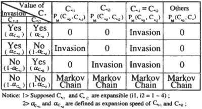
As respect to class change by temporal continuity under the effect of expansion-contraction, all possible patterns of class change are listed in Table.1. From this table, we can determine the probability of class changes by temporal continuity under the effect ofexpansion-contraction, PTC(CI, C.), based on the probability of class changes in Markov chain PM( Coo, ' C. ) , and the expansion speeds if the invasion of neighbouring pixels is happened. All behaviors of class change under the effect of expansion-contradiction can be deduced from the table like Table.2.
|
C*0
C*0'S neighbours |
unshinkable | unshrinkable |
| unexpansible | Markov chain | Markov chain |
| expansible | Markiv chain | Markov chain + Invasion |
3.4 Definition of Operators
3.4.1 Reproduction
Reproduction is a process in which individual strings are copied according to their objective function values or the fitness values. Copying strings according to their fitness values means that strings with a higher value have a higher probability of contributing one or more offspring in the next generation(Figure.4). This operators, realizing an artificial version of natural selection, a Darwinian survival of the fittest among string creatures.
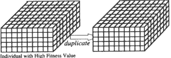
Figure 4 Reproduction of Individual
There are several proposals for selecting survival individuals. The most basic scheme are called the roulette wheel scheme, the deterministic sampling and the elitist scheme. In order to efficiently find the best solution in search space, in our search, we proposed the selection scheme based on the combination of the deterministic sampling and the elitist scheme. The selected survival possibility in next generation of each individual is calculated as in the deterministic sampling. And the best individual is kept into the next generation as in the elite scheme.
3.4.2 Crossover
Crossover operator first randomly mates newly reproduced individuals in the mating pool. Then it randomly locates a Window with random size for a pair of individuals. Finally, the contents of individuals within the window are swapped to create new individuals (Figure.5).

Figure.5 Crossover of Individuals
3.4.3 Mutation
Mutation operator plays a secondary role in the simple GA. It occasionally alters the value in a individual position (Figure.6).
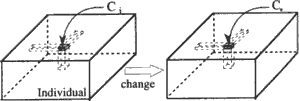
Figure.6 Mutation of One Individual
4. Improvement of the Search in Genetic Algorithms
4.1 Hill-Climbing method to improve the efficiency of genetic algorithm
Searching a complex space of problem resolutions often involves a trade-off between two apparently conflicting objectives: exploiting the best solutions currently available and robustly exploring the space(Lashon Booker, GA&SA). Generic algorithms have been toured as a class general purpose search strategies that strike a reasonable balance between exploration and exploitation. The power of these algorithms is derived from a very simple heuristic assumption: that the best solutions will be found in 1- regions of the search space containing relatively high proportions of good solutions. The problem is that, ..if the complex space of problem resolutions become larger and larger, the population size and the generation size have to be increased at same time. The efficiency of GA is one of obstacles to apply GA in reality.
Hill climbing is a good example of a search strategy that exploits the best among known possibilities for finding an improved solution. Although Hill-Climbing strategies is easy to trap in one of local maxima more far away from the optimal solution, it is a very good search strategy that exploits the best among known possibilities for finding an improved solution. So in our research we try to combine the Hill- Climbing strategy with GA.
4.2 Maintenance of Population Diversity
Despite the demonstrated advantages of GAs and high performance of most implementations, it still fails to live up to the high expectations engendered by the theory. The problem is that, any implementation uses a finite population or set of sample points. Estimates based on finite samples inevitably have a sample error associated with them. Repeated iterations of algorithm compound the sample error and lead to search trajectories much different from those theoretically predicted. The most serious phenomenon is the premature convergence.
The premature convergence is caused by early emergence of an individual that is better than the others in the population, although far form optimal. Copies of this structure may quickly dominate the population. Search continues then but is concentrated in the vicinity of this structure and may miss much better solutions elsewhere in the search space.
To avoid the premature convergence, one has to maintain population diversity or to reduce the different of best fitness with others. Although, to reduce the reproduction number can not eliminate the premature convergence, it can be used as a simple way to reduce the rapid convergence. Therefore, in our research, we limited the duplicated number of individuals within two. It means that if individual's expected duplicated number is larger than two, we will force it to equal two. To do so, the premature convergence speed can be reduced.
5. Experiment
The test program of GNHC for spatio-temporal interpolation of pixel based landuse data was coded with C language and was run on SP ARC/station2. Several simple landuse class variable data had been used to test program. For the test data, only two dimensional spatio-temporal data is shown here. The test data size of individual had been defined with 20pixels*6time-slices. The first and last time-slice in the individual were supposed to be sampled data and all middle time slices were unsampled data which needed to estimate through interpolation size processing. In these experiments, we set the generation size of GA/HC to 2000,which was large enough to get stable results. The probability of crossover operation was definded as 0.7, while the probebility mutation operation was relative small in natural population, so that we used 0.01 as the Time Boundary condltlon probability of mutation. Figure.7 is one of experiment results of GA/HC, in which the individual has largest fitness value.
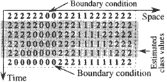
Figure 7 Result of GA/HC
Figure.8 shows the comparison of several experiment results From this figure, we can find that the larger the population size is the faster the stable result can be obtained, and the closer the stable result tend to best solution. Figure.9 is a comparison of GNHC with GA for spatio-temporal interpolation of landuse class variable data. It shows GA/HC has much higher efficiency than GA for GA spatio-temporal interpolation.
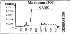
Figure 8 Comparison of GA with GA/HC
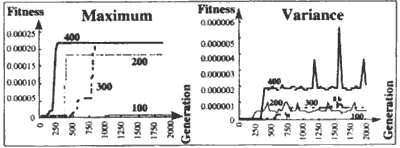
Figure 9 Effect of Population & Generation Size
When observed location of class '0' in the first time slice and the last time slice are overlapping spatially, the Interpolation result naturally connect class '0' together, as shown in Figure.l0, forming a band of class '0' .On the other hand, if class is not overlapping spatially, the most likely interpolation result do not connect class '0' together as in Figure.ll, while the case forming a band of class '0' apparently have lower likelihood, though it looks natural. In Figure.12, another observational data is given at the middle. In this case, the most likely spatio-temporal pattern of class changes has a band of class '0' .It means that the interpolation methods integrating observational data and behavioral models can update the most likely results dynamically whenever new observational data are given.

Figure 10 Interpolation Result in Overlapping Case

Figure 11 Interpolation Results in Unoverlapping Case
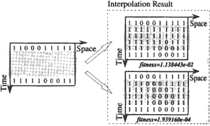
Figure 12 Interpolation Result with Additional Observational Data
6. Conclusion and Future Prospects
In this study, Genetic-Algorithm/Hill-Climbing was proposed as a spatio-temporal interpolation scheme for pixel based class variable data which allows integration with observational data and behavioral/ structural models/rules. Test experiments can be summarized as following:
- GA/HC can be very rigorous because it can generate the most likely spatio-temporal distribution of class variables under observational data and a behavioral model;
- Hill-Climbing method can be effective method to greatly improve the efficiency of GA;
- Bramlette, M.F. (1991): Initialization, Mutation and Selection Methods in Genetic Algorithms for Function Optimization, Proc. of the 4th. Conf. on GA, R.K.Belew and L.B.Booker (Editors), July, 1991, pp.loo-107.
- Burrough, P.A. (1986): Methods of Spatial Interpolation, Principle of GIS for Land Resource Assessment, Monographic on Soil and Research Survey, No.12, 1989, pp.147-166.
- Davis, L. (1987) : Genetic Algorithms and Simulated Annealing, Pitman Publishing, 128 Long Acre, London WC2E 9AN, 1987.
- Davis, T.E., J.C.Principe (1991) : A Simulated Annealing Like Convergence Theory for the Simple Genetic Algorithm, Proc. of the 4th Conf. on GA, R.K.Belew & L.B.Booker (Editors), July,1991,pp.174- 181.
- Eshelman, L.J. and J.D.Schaffer (1991): Preventing Premature Convergence in Genetic Algorithms by Preventing Incest, Proc. of the 4th. Conf. on GA, R.K.Belew and L.B.Booker (Editors ), July, 1991, pp.115-122.
- Goldberg, D.E. (1989) : GENETIC ALOGRITHMS in Search, Optimization and Machine Learning, Addison-Wesley Publishing Company, Inc., 1989.
- Gold, C.M.(1989): Surface interpolation, spatial adjacency and GIS, Three Dimensional Applications in Geographic Information System, Edited by J.Raper, Taylor & Francis Ltd., 1989, pp.22-35.
- Huang, S.B. and R.Shibasaki(1995): Development of Genetic Algorithm /Hill-climbing Method for Spatio-temporal Interpolation, The 6th Symposium on Functional Image Inf. System, lIS, Univ. of Tokyo, Apr. 1995, pp.81-86.
- Shibasaki,R., T.lto and Y.Honda (1993): Integration of Remote Sensing and Ground Observation Data for Developing Global GIS, Proc. Of SElKEN Symposium, Vol.12, Aug. 1993, pp.263-277.