GISdevelopment.net ---> AARS ---> ACRS 1998 ---> Poster Session 3 Density and Temperature Profile in the Lower Atmosphere at Kmitl, Thailand Sokkiat Lerkvaranyu, Kobachai Dejhan, Fusak Cheevasuvit Faculty of Engineering and Research Center for Communication and Information Technique, King Mongkut's Institute of Technology Ladkrabang, Ladkrabang, Bangkok 10520, Thailand Tel-: 66-2-3269967, 66-2-3269081, Fax : 66-2-3269086. E-mail: kobchai@telelan.telecom.eng.kmitl.ac.th Toshikasu Itabe, Kohei Mizutani Toshikasu Itabe, Kohei Mizutani Communication Research Laboratory Nukui-Kitamachi 4-2-1, Koganei, Tokyo 184, Japan Tel : 81-423-27-7546, Fax : 81-782-7094 Abstract Continuously, the developed of lidar system at The King Mongkut's Institute of Technology Ladkrabang (KMITL) is ex tended. The ability of laser radar to measure the density and temperature profiles by the method or Rayleigh scattering also called Rayleigh lidar. An 180 mJ Nd: YAG laser at 532 mm wavelength and 28 cm diameter of Schmidt-Cassegrain telescope the density and temperature profiles in the lower atmosphere are installed. The density profile can be indirectly obtained from lidar equation, the temperature profile will be obtained from hydrostatic equation. Finally, the results of density and temperature profiles seldom relate to phenomenon profile that obtained from radiosonde. The paper proposes to measure the density and temperature profile in the lower atmosphere at KMITL, these data will be used for the other purposes. Introduction To study the behavior of atmosphere, he various lasers were applied after the laser was invented. The atmospheric is very complicated system so the used of laser to study it has many type such as the measurement of ozone, vapor water, cloud, fox and etc., including the aerosol measurement in boundary layer. Those laser system can be called the atmospheric laser radar or synonym the lidar system and has the various techniques of signal processing depend on the purpose of measurements to attract the specific information that come from with the return signal. For the measurement of the number density or the number of a mixture of gases, the used technique is Rayleigh lidar in which he signal can be obtained mainly from the elastic backscattering of the laser energy by any particles in the atmosphere. Moreover, in the Rayleigh technique, it may be use multiwavelength simultaneous for the comparison the different characteristic that effect from the mixing particle. It should avoid the comparison the different characteristic that effect from the mixing particle. It should avoid the absorption band because this technique only use the backscattering. For a single wavelength the Rayleigh technique can also be used but the accuracy will be decrease for more detail see in reference[3]. Considering the Rayleigh technique for measuring the number density, the number relationship of various gases in atmosphere will be different. If the considered altitude is troposphere or boundary layer, the mixture of gases is homogeneous and a little different. The number of whole gases in the atmosphere closed to a model with respect to the altitude. Nevertheless, it has many atmospheric model and one well-known is the U.S. standard atmospheric model. To assume the mixture of various gases in lower atmosphere is homogeneous so that the average weight and mean molecule number can be obtained. The return signal occurs from scattered the particle in any altitude can be calculated from cross section value of the average number density. It means that the number density can be derived from observation data. It has several methods that convert the return signal to number density, for more detail as in reference [2,3]. Importance, the number density that obtain from return signal is not only the mixture of various gases but also include the aerosol and any particle in the atmosphere. In the volume is constant, the ideal gas law has the relationship with pressure, temperature and molecular number and the hydrostatic equation shows the relationship between pressure and temperature in the equilibrium assumption. It is possible to determine the temperature profile. However, it should care the limitation of this method because the error occurs from the scattered signal from other particles, especially in the boundary layer which ha many aerosol, thin cloud and so on, it can increase the return signal. Lidar system In the experiment, the system is monostatic Rayleigh lidar that means the transmitter and receiver is located in the same place. The transmitter is the Nd: YAG laser that emit he second harmonic wavelength (532 nm) and the laser beam is transmitted in the vertical axis with respect to the earth. And, the received uses the telescope with 28 cm diameter that will collect the scattered laser light from molecule and any particle in the field of view of receiving telescope. The collected light by telescope will focus on a photomultiplier which converts the energy to be electrical signal. Consequently, in the optical remote sensing the photon counting techniques is helpful when the return signal is very weak. Finally, the photon counting signal will be transferred to a personal computer were the signal will be processed and analyzed. The detailed system is shown in Table 1. Table 1. Characteristics of Lidar system Transmitter Laser Nd. YAG, SHG (532 nm) Output 180/mJ/p Repetition 10 Hz Beam div 0.1 mrad Receiver: Telescope Sehmidt-Cassegrain 28 cm diameter Detector PMT, S-1 R3236 Hamamatsu Signal and data analysis As the telescope receives the scattered light in according to the transmitted laser light in the field of view of receiving telescope. The ground-based monostatic radar will be in this experiment. Usually, the optical remote sensing equation describes as follows, N(z) = [hT2] [Plt/hc] [lb(z)n(z)DZ] [Ar/4pZ2]+ [Npt]  (1) N(z) is expected number of photons detected in the interval DZ , n(z) is particles density of range Z, Nn are expected photon due to background noise, DZ is receiver range bin length, Ar is the telescope aperture area, l is optical wavelength, h is Plant's constant, c is light velocity, P is laser power, T = exp[-Ss(z)DZ] is one-way transmittance where s is the extinction cross section, R is laser pulse rate, t is integration time, h is system efficiency and b(z) is effective particles backscattering cross section converts to be the number of density via the relation of average molecule with cross section at this wavelength. To determine the temperature from the lidar density profile is integrated upward or downward using the hydrostatic equation and the initial temperature may be obtained from a model or local temperature as integrate upward. The normally hydrostatic equation is dP = -pg dz    (2) And the ideal gas law is P = rRT -------- M    (3) Finally, the integrated temperature equation is T(z) is the atmospheric temperature profile, P(z) is atmospheric pressure profile, p(z) is density profile, g(z) is the gravitational acceleration, M is mean molecular weight of the atmosphere, R is universal gas constant is the altitude of temperature estimate. 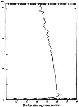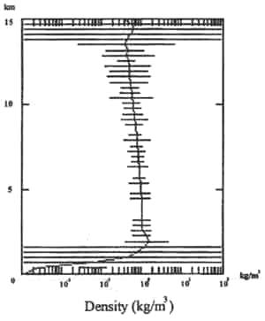Result Figure 1 shows the relation between the backscattering cross section which obtain from data in log scale with altitude. After obtaining backscattering cross section, the density profile that convert from backscattering cross section profile. However, the error will be occur because the return signal that come from both mixture of various gases and the aerosol or any particle in the atmosphere so that the density profile is the average of the collection of return signal. Figure 2 illustrates the averages density with the line of standard deviation at any altitude. Figure 1. Backscattering cross section Figure 2. 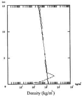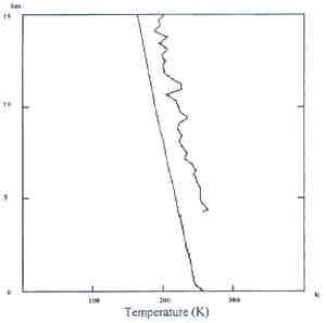Average density Figure 3. show the comparison between the density profiles which obtains from the observation and a direct line by simulating from U. S. model. Figure 4 is the temperature that come from integrated hydrostatic equation. Moreover, in the figure 4 also compares the temperature from the observation with a direct line that come from with model. Finally, the three-difference of temperature value come from observation, model and radiosonde, respectively, as show in the Table 2. Figure 3. Density which obtain from observation and simulation. Figure 4. Temperature profile Table 2. Three-difference temperature value Altitude (m) U. S. standard (K) Observation (K) Radiosonde (+ m) 900 282.30 - 295.35 (+9) 1800 276.45 - 290.15 (+75) 2700 270.60 - 285.55 (-65) 3600 264.76 - 280.65 (-75) 4500 258.93 287.89 275.25 (+108) 5400 253.08 284.58 271.85 (+38) 6300 247.24 278.04 276.85 (+38) 7200 241.40 265.62 260.95 (-33) 8100 235.56 258.69 254.05 (+120) 9000 229.73 267.66 248.45 (+84) 10800 218.06 257.23 234.15 (+93) 11700 216.65 232.19 228.55 (-154) 12600 216.65 238.72 219.05 (+48) 13500 216.64 219.30 211.75 (+25) 14400 216.65 221.29 205.95 (-131) Summary The lidar system at KMITL has been developed continuously. In this paper, the number density profile and temperature profile are determined. For troposphere or boundary layer, it is difficult to obtain the number density and temperature profile correctly because the Rayleigh lidar method uses for the backscattering, but the boundary layer has many various particle, especially the aerosol and cloud that will cause the error. However, this method is useful for the stratosphere or higher altitude. References J. D. Klett, J. Appl. Opt., vol. 20, pp. 211-220, 1981. R. M. Measures, Laser Remote Sensing: Fundamentals and Application NewYork, NY: Wiley, 1984. P. B. Russell and B. M. Morley, J. Appl. Opt., vol 21, pp. 1554-1563, 1982. F. G. Fernald, J. Appl. Opt., vol. 23, no5, pp. 652-653, 1984. F. G. Fernald, B. M. Herman and J. A. Reagan, J. Appl Meteoro., vol. 11, pp. 482-489, 1972. B. R. Clamesha, G. S. Kent, and R. W. H. Wright, J. Appl. Meteoro., vol. 6, pp. 386-395, 1967. K. Parameswaran, K. O. Rose, and B. V. Krishna Murthy, J. Appl. Opt., vol. 30, pp. 3059-3071, 1991.