Choice of the Best Band Combination of Hyper spectral Data

Choice of the Best Band Combination of Hyper spectral Data

Liu Jianbo
China Remote Sensing Satellite Ground station, Academy of Science, 100086
E-mail:http://www.gisdevelopment.net/aars/acrs/1999/ps6/jbliu@ne.rsgs.ac.cn

Abstract
Hyper spectral remote sensing data of many channels, some have hundreds. When display or hardcopy of this kind of data is needed, hyper spectral data users are often confronted with the following question: How to choose 3 channels for RGB combination from so many channels to get the best visual effect?

A method of low to choose the best band combination of hyper spectral data is discussed here. Through mathematical calculation, this method considers high divergence degree and least correlation channels as best band combination. An example study for AVIRIS data (224channels) shows its remark power. And more, because the method is ground feature oriented, it is application for different hyper spectral data users with different application needs.

Introduction
One major advance in remote sensing technology in the past decade is hyper spectral remote sensing. The Jet propulsion Lab (USA) has produced two Hyper spectral sensors, one known as AIS first flown in 1982, the other as AVIRIS (Airborne visible/Infrared Image Spectrometer) which continues to operate since 1987. AVIRIS consists of a total of 224 channels. Europe, China and Japan also have their own experimental hyper spectral imaging system.

The potential uses of hyper spectral data have been studied in various areas, especially in mineral and vegetation distinguishing. Quite a few impressive result have been reported. Some new hyper spectral imaging system will go into operation soon.

When utilizing hyper spectral data, users usually need a special image processing software, like ENVI, which is able to processing and display multi channel information. With the help of this kind of software, researchers could then analyze the spectral characteristic of ground features and get the solution for their application.

In remote sensing image processing, users have often to choose 3 band for display of hardcopy.

For data with fewer bands, like TM, it is not a difficult task. The common RGB combination for TM is 432, 742,453,etc not so easy a job to choose 3 channels for RGB combination to get the best visual effect from hyper spectral data, which have tens of hundreds channels. To solve this problem, we have developed a method in our work. The method takes both channel correlation and divergence degree factors into account.

Method
Obviously, the best band combination varies with application object. Different user have different requirement. Botanists mainly want to distinguish the vegetation, while mineralogists pay much attention to the difference between minerals. They will choose different band combination for display or printing. Hence, when choosing best band combination, user have to9 first determine the ground feature they concern. We call it target ground feature. If users, for example, concern bare land, forest, grass land, snow, and water body, best band combination should have them shown contrast sharpest.

Best band combination should make use of the characteristic of hyerspectral data. Hyper spectral data has many channels. Every channel has a very narrow band width, 10 nanometer for AVIRIS as an example. For any given ground feature, when plotted as intensity versus wavelength a meaningful spectral curve can be drawn through the sufficient number of points. This means when target ground feature determined , its spectral curve is also determined. The best band combination is chosen according to the shape of the spectral curve and the relationship among them. The basis rules we set are:

The best band combination should be composed of channels with the greatest divergence degree.

In a chosen channel, the intensity of target ground feature should be separated from each other as even as possible. Suppose N ground feature have been selected as target feature. I_max and I_min are, respectively, the maximum and the minimum intensity of these N feature in a channel. Let K=(I_max -I_min) /2N. If the intensity difference between two features is greater than K, these two ground feature are then considered as divergent to each other in this channel. It is easy to each other in this channel. It is easy to infer that the greatest possible divergent pairs for N ground feature is (N-1)+…….+3+2+1. We define the divergence degree as the ratio of actual divergent pairs to the greatest possible divergent pairs. Calculation according to the above definition, we could get target ground feature divergence degree in every channel. The best band combination should be composed of channels with great divergence degree, for example, channels with divergence degree equal or greater than 0.9.
As far as the target feature are concerned, the correlation degree among 3 selected channels should be smallest.

Hyperspectraldata data has a very high spectral resolution. If the target ground feature divergence degree in channel m is great, the divergence degree in channel in its neighbor channels (channel m-1and channel m+1) will generally also great. Obviously the combination of these 3 channels will produce a nearly black& white image. We should not choose these 3 channels as RGB combination band. They are too much similar. In another word , they are too much correlative. So, in addition to divergence degree condition as stated above, the best band combination between the selected channels.

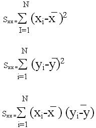
Suppose the intensity of N target ground features in channel m and channel n area x₁, x₂, ... ... , x_N and y₁, y₂, ... ... , y_N respectively. According to mathematical correlation theory, we have

r_xy is correlation coefficient , while

The correlation coefficient between every 2 channels could be calculated with the formula. Since the best band combination is composed of 3 channels ( 1, m,n) should be chosen is a minimum. That is to say, r_lm+r_ln+r_nm is a minimum.

Example
Here we use an AVIRIS hyper spectral data to show how the above method works.

Selected channels with greater divergence degree as candidate channels for the next input. In this test we set divergence degree ³0.9. Among all of 224 channels, 79 channels agree with the condition. We then calculate the correlation coefficient between every 2 channels among these 79 channels For every possible 3 channels combination,

The data is line 512 by pixel 664 by 224. Flight number: 940719B. Run 9. Acquired time: July 19,94. Area: Cascade, Washington, USA. Scene center latitude: N48:31:56, longitude: W121:23:54.

First step is to choose target ground features. This could be done as follows. Read the test data into ENVIsystem. Display the image using 3 channels at random, better one in green waveband, one in red waveband and one in infrared waveband. Point the concerned ground features with mouse and record the value associated with it.

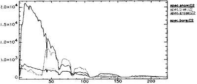
For this example we choose bare land, forest, grass land, snow, and water body as target ground features. Now we have the 224 intensity value for every target ground feature. The spectral curves of them are shown in figure1 (color). The intensity, K value, and the divergence degree of these 5 target features in some typical channels are shown in Table 1.

Figure 1(col). Spectral curve of the 5 target ground features
Sum up the 3 correlation coefficient. Then sort all of the sum from minimum to maximum. The combination at or near the top are the best band combination. Table 2 mainfests the ten least correlative degree combination from all the channels with the divergence degree ³0.9. These are the ten best band combinations.

Table 1. The I, K and Divergence Degree Of the 5 target feature in some typical channels

CH	I_bare	I_show	I_forest	I_grass	I_water	I_max-I_min/2N	DD
2	1516	2889	549	562	813	234	0.9
24	2656	18279	1035	1386	4360	1724.4	0.6
60	1447	4952	1567	4689	207	474.5	0.8
71	1771	3141	1786	5275	117	515.8	0.9
175	165	.7	10	15	9	15.8	0.4

CH……..Channel DD………Divergence Degree
Table 2. The top best band combinations

CH1	CHm	CHn	DD1	DDm	DDn	r_lm+r_ln+r_nm
2	71	126	0.9	0.9	0.9	0.404684
2	70	126	0.9	0.9	0.9	0.405569
2	72	126	0.9	0.9	0.9	0.409384
2	69	126	0.9	0.9	0.9	0.420881
2	73	126	0.9	0.9	0.9	0.421018
2	71	127	0.9	0.9	0.9	0.441627
2	70	127	0.9	0.9	0.9	0.442508
2	68	126	0.9	0.9	0.9	10444903
2	72	127	0.9	0.9	0.9	0.446218
2	74	126	0.9	0.9	0.9	0.447456

CH ...Channel DD ...Divergence degree
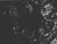
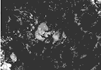
Among the combination with sum of correlation coefficient bigger than 0.404486 and smaller than 2.0, we have chosen more than a hundred combination for comparison. The result is remarkable. The combination at or near the top of lost have very good display effect, with bright color and sharp contrast for the selected target feature. It clearly shows the following general rule: The smaller the sum of correlation coefficient is the better the image looks. The results of 2 typical combination are shown in figure 2 (color) and Figure3 (color).

Figure 2(col). CH126(R)71(G)2(B), Sum of correlation coef=0.404684

Figure 3(col). CH69(R)46(G)2(B), Sum of correlation coef=1.489137
Conclusion and Discusion

The method discussed above take the following two important factors, spectral curve divergence degree and channel correlation degree, into account. The result shows the RGB band combination chosen based on these principles is effective.
Because the method is ground feature oriented, it is applicable for different hyper spectral data user with different application needs.
The divergence degree threshold value is adjustable. If the candidate channels for correlative calculation are too few, the divergence degree threshold value could be set to a lower value.
Target ground feature can be sampled either by point or by small area. We prefer by area for its average effect.
Channel 1, channel 107-113, channel 154-167, and channel 221-224 of raw data area bad data. They are not considered during the calculation.

References

Rothery, D.A., Decor relation stretching as an aid to image interpretation International Journal of Remote Sensing, Vol. 8.